Conclusion
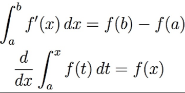
Now that we've covered both FTC part 1 and part 2, hopefully you understand how an integral and a derivative are related to one another.
Recap:
FTC Part 1 allows us to find the total distance a ladybug crawls along a leaf by adding up small rectangles of equal subintervals. This is also known as accumulating the area under the curve. By doing this, we find how far a ladybug travels between the time interval [a, b].
FTC Part 2 tells us we can use f(t) and t as dummy variables until we substitute x into the function. Thus, we can choose an x between a and b to find specific distances covered by the ladybug. Part 2 also conveys that the integral and derivative are inverses of each other which is why we can substitute x directly into f(t). This allows us to find the distance covered between different time intervals. By adding or subtracting these intervals (or areas) together, we can create expressions about the distance a ladybug covers over time.
How can we use this information to further investigate other mathematical topics?
What if we had a function f(x, y) such that it had two variables instead of just x? That is, it takes up multiple dimensions instead of just 2D?
Although most high school students are in AP or BC Calculus classes, multivariable calculus begins dealing with functions in 3D and 4D.
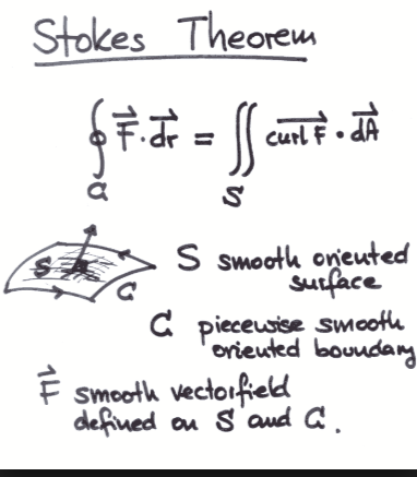
Consider Stoke's Theorem:
Consider f(x, y) which is a figure on the x, y, z plane. Then, there is a surface since it is multidimensional with curve C being the outer boundary of this figure.
When we just dealt with f(x), it was a curve through space, but now we have a figure in space. Thus, there is a surface area involved now.
What Stoke's Theorem allows us to do is similar to the Fundamental Theorem of Calculus. Simply put, we can find the individual derivatives between a starting and ending point that allows us to find the surface area of the figure.
While this sounds confusing, let's consider a simple 3D diagram example. In the past, we have found a tangent line to a curve. That is, there was a specific point on a curve created by f(x), and we used a tangent line to find the instantaneous rate of change at that point. Now, our starting point is beginning at some point on the outer boundary of our shape. Looking at the diagram above, the curve of C is the outer boundary of shape S. How can knowing the individual derivates around C help us find the surface area?
Futher, now that we are dealing with shapes in 3D, we can no longer use a tangent line. Instead, we use a plane!
What if we had a function f(x, y) such that it had two variables instead of just x? That is, it takes up multiple dimensions instead of just 2D?
Although most high school students are in AP or BC Calculus classes, multivariable calculus begins dealing with functions in 3D and 4D.
Consider Stoke's Theorem:
Consider f(x, y) which is a figure on the x, y, z plane. Then, there is a surface since it is multidimensional with curve C being the outer boundary of this figure.
When we just dealt with f(x), it was a curve through space, but now we have a figure in space. Thus, there is a surface area involved now.
What Stoke's Theorem allows us to do is similar to the Fundamental Theorem of Calculus. Simply put, we can find the individual derivatives between a starting and ending point that allows us to find the surface area of the figure.
While this sounds confusing, let's consider a simple 3D diagram example. In the past, we have found a tangent line to a curve. That is, there was a specific point on a curve created by f(x), and we used a tangent line to find the instantaneous rate of change at that point. Now, our starting point is beginning at some point on the outer boundary of our shape. Looking at the diagram above, the curve of C is the outer boundary of shape S. How can knowing the individual derivates around C help us find the surface area?
Futher, now that we are dealing with shapes in 3D, we can no longer use a tangent line. Instead, we use a plane!
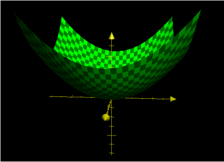
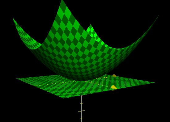
Consider the following function f(x, y) = x^2 + y^2
This can also be written as z = x^2 + y^2 because we are in 3D. Thus, we now have 3 variables: x, y and z.
This figure is called an elliptic paraboloid. It's a fancy word for describing a shape that opens upward like a parabola but also has the shape of an ellipse.
This can also be written as z = x^2 + y^2 because we are in 3D. Thus, we now have 3 variables: x, y and z.
This figure is called an elliptic paraboloid. It's a fancy word for describing a shape that opens upward like a parabola but also has the shape of an ellipse.
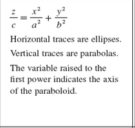
We notice this by the following equation (Steward Calculus Textbook):
Now, we want to find a plane tangent to a point on this figure. Let's choose (0, 0, 0), the origin to make this simple.
How can we find a plane that is tangent to the origin?
We want a flat surface that has no height since we want it at the origin. However, it should cover the x and y axis. Thus, the x and y coordinates can be any value, but z should be zero since our figure should have no height.
|
Thus, let z = 0. Now, we've created a plane going through the origin (0, 0 , 0)!
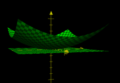
But how do we know it's actually tangent to the figure? By zooming in, we can determine this. |
|
|
|
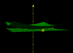
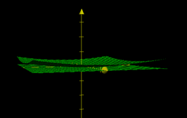
As we continue zooming in on our graph, we notice that the elliptic paraboloid becomes flatter and flatter. Thus, its shape is becoming more similar to our plane at z = 0. Thus, z = 0 is tangent at the origin.
If this part is confusing, don't sweat it! It's definitely more advanced. But it's pretty cool to see how ideas from the FTC can be used in more complex mathematics.
If you're still shaky on any concepts, feel free to revisit any pages!
If this part is confusing, don't sweat it! It's definitely more advanced. But it's pretty cool to see how ideas from the FTC can be used in more complex mathematics.
If you're still shaky on any concepts, feel free to revisit any pages!