Derivatives and Limits
What is differentiation? Putting it in simple terms, deriving means finding the slope of a line tangent to a function.
One way to think of this is as the slope of a curve. Why does knowing the slope of the curve matter? We briefly discussed this on the Accumulation and Rates of Change page. If you're still confused, revisit that page!
We know that the rate of change is the same as slope, and we've talked about two kinds of slope. Which one is most relevant by looking at the picture to the left? That is, which type of slope would best help us find the distance covered by the ladybug?
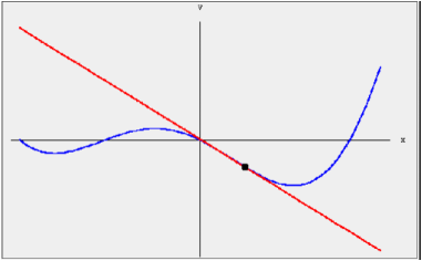
Looking at this geometrically, let f(x) be the blue curve on the graph. The red line is the tangent line to the blue function curve. It is "tangent" to the specific point in black (this means it represents the instantaneous rate of change!)
Refer to the following website and scroll down until you see the third graph with the
green tangent line: http://www.sosmath.com/calculus/diff/der00/der00.html
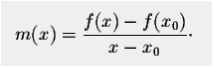
Here, the original point on the blue curve is sitting idly. Let's call this point A. We can see that the green line also contains a point in black, so let's call this point B. Overtime, point B moves closer to point A until eventually, it's literally sitting on top of point A. This is where the point slope formula comes from. The formula requires two different points: a beginning and an end point. The tangent line itself has a slope m which follows the equation below:
One way to think of this is as the slope of a curve. Why does knowing the slope of the curve matter? We briefly discussed this on the Accumulation and Rates of Change page. If you're still confused, revisit that page!
We know that the rate of change is the same as slope, and we've talked about two kinds of slope. Which one is most relevant by looking at the picture to the left? That is, which type of slope would best help us find the distance covered by the ladybug?
Looking at this geometrically, let f(x) be the blue curve on the graph. The red line is the tangent line to the blue function curve. It is "tangent" to the specific point in black (this means it represents the instantaneous rate of change!)
Refer to the following website and scroll down until you see the third graph with the
green tangent line: http://www.sosmath.com/calculus/diff/der00/der00.html
Here, the original point on the blue curve is sitting idly. Let's call this point A. We can see that the green line also contains a point in black, so let's call this point B. Overtime, point B moves closer to point A until eventually, it's literally sitting on top of point A. This is where the point slope formula comes from. The formula requires two different points: a beginning and an end point. The tangent line itself has a slope m which follows the equation below:
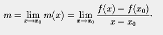
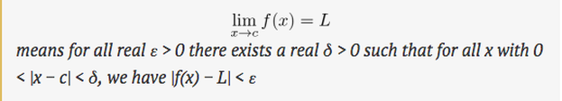
As the two points become closer and closer together, we can find a more precise slope. This is where average velocity and instantaneous velocity differ. The average slope (or rate of change or velocity) is between two different points while the instantaneous velocity is the velocity at a specific point and time equal to the specific slope of the position. The difference between the two is best explained through limits. The image to the right may look intimidating, but we can walk through this slowly!
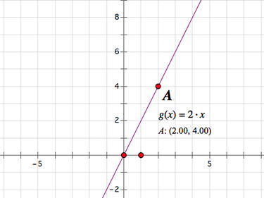
Let's look at the following video below. Here, we have the function f(x) = x^2 with a point plotted at (2, 4). We choose (2, 4) because we know that 4 is the derivative when x = 2. How do we know this? Try taking the derivative of f(x). What do you get?
Then, substitute x = 2 into the equation.
While looking at the video, we have an arbitrary point B located on the f(x) curve. As we watch the video, point B moves closer and closer to point A = (2, 4). By looking at the slope of the line AB, we can see that eventually point B passes through the y-value 4. So, we begin with the average rate of change, but as the limit becomes closer and closer to 4, we see that the AROC = IROC. Thus, taking the derivative and substituting in an x-value gives us the instantaneous rate of change. We can also visualize this with the use of limits!
As stated previously, as two points move closer and closer together, the actual value of the y-value on the graph becomes more specific. The limit tells us what y-value we are approaching as we become closer and closer to the same x-value. Here is the actual definition of a limit. It is scary sounding, but using this interactive activity will be very helpful in visually understanding what it means! http://stevekifowit.com/geo_apps/limits_2.html
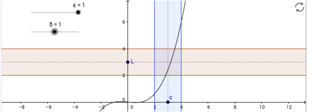
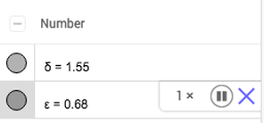
Once you go the website, you will see sliders for the epsilon and delta values. To begin, set both equal to 1 and see how large the width of each is. We can see that this takes a large chunk of the curve into consideration. We can now try sliding both to .25. What changes do you notice?
Something else to try with this activity: on the left side, click on epsilon and delta in their respective tabs and press the "play" button. You can then watch the sliders move on their own and watch how the width of each increases and decreases. How does this play a factor in determining the limit of a function at a specific x-value? Are you able to see how the definition of a limit can be visualized? Spend some time changing the function of x and watch how the epsilon and delta variables fluctuate.
This helps us visualize how limits specify how far the ladybug has crawled along the leaf! If you're ready, click here to learn about inverses.