Continuing on the idea of using a smaller delta x, we can think about the fundamental theorem of calculus geometrically as well. We will use something called Riemann sums to help us visualize this. In fact, we will be creating two different kinds of approximations to help us estimate the total distance traveled by the ladybug. Refer to the following website (Renault, Marc).
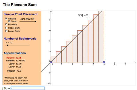
On the left hand side towards the bottom, there is a slot to type in a function. Let's let f(x) = x for simplicity sake. This will allow us to see a straight line beginning at the origin. This will represent the ladybug's path. Now drag the blue/purple dots at the x-axis so that we are only looking at x values between x = 0 and x = 5. If we set the subintervals equal to 10, we will see 10 rectangles taking up that space between x = 0 and x = 5. This allows us to approximate the total area underneath the curve of f(x) = x.
By creating 10 rectangles, we are taking the total time the ladybug is crawling and splitting this up into 10 equal time lengths. This helps us determine how far the ladybug is able to crawl within our set time period.
You should be able to see that the actual integral is 12.5, but the estimates are slightly higher and/or lower than this. This is based off of two different approximations that we will talk about: left hand Riemann sums (LHRS) and right hand Riemann sums (RHRS).
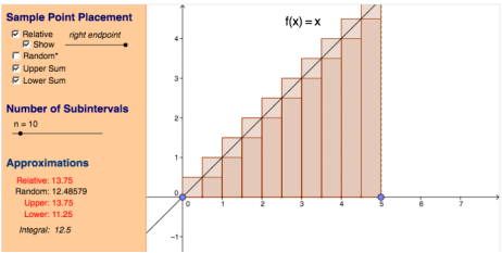
The LHRS works as such: begin on the left side along the y-axis and draw a rectangle so that when you move your cursor to the right side, it will hit the f(x) curve (the function's curve). This should happen at approximately x=.5. You then draw a straight line directly down to the x-axis. That is your first rectangle. Continue to do this until there are 10 evenly spaced rectangles between x = 0 and x = 5. The LHRS is shown by the lighter colored rectangles.
RHRS: we start from the right side (x = 5) and move our cursor to the left as we make 10 even rectangles until we get to x = 0. For the first rectangle, move your cursor to the left until you touch the f(x) curve and then draw a straight line down to the x-axis. This is illustrated by the darker colored rectangles.
The LHRS and RHRS rectangles are highlighted in the picture to the right. Notice that the LHRS creates rectangles that are above the curve. Stop for a moment and think about this! What does this mean in terms of adding pieces of area together?
(This means we are taking in more area than we should be, so the estimation will be "more" than the actual integral).
For the RHRS the rectangles are under the curve, so we are underestimating more than we should be. So, does this mean we are estimating more or less than the actual integral?
Unfortunately, this website does not explicitly say left hand and right hand, but the "Upper" refers to the left hand Riemann sum and the "Lower" refers to the right hand Riemann sum.
Now, try increasing the subintervals and notice what happens to the estimations in comparison to the actual integral. Also, compare the estimations to when the number of subintervals was n=10. What do you see happening? Why do you think this is?
What does this mean when we break our time interval up into more even pieces? How does this affect the error of how far the ladybug travels?
This website helps us understand the idea of accumulating the area under the curve in the form of rectangles from a specific starting point to an ending point. By doing so, we find the total distance that the ladybug crawls, and we can think of this as adding the distance covered one rectangle as a time until we find the total distance that the ladybug has traveled from [a, b].
We can relate this to accumulation and rates of change to better understand FTC part 1. If you're ready, click here.
